The Math of Teaching a Robot Dog to Walk (and Why It First Learned to Stand Still)

Part 1 of a series on training a simulated Unitree Go1 quadruped with reinforcement learning. Everything here comes from runs on a single RTX 5060 (8 GB) with MuJoCo Playground, MJX/Warp and Brax PPO.

We trained a four-legged robot to walk from scratch. Nobody told it how legs work. It got no motion capture, no reference gait and no demonstrations. It had a physics simulator, a neural network and a number that went up when it did the right thing.

The first time we trained it, the number went up and the robot learned to stand perfectly still and spin in place. That failure turned out to be the best way to understand the math, so this article builds up the machinery and then uses it to explain exactly why the robot got stuck, and how it got out.

1. The problem, written down

Reinforcement learning frames control as a Markov decision process (MDP):

M=(S,A,P,r,γ)

$s_{t} \in S$ : The state of the world at step $t$ (every joint angle, velocity, and contact).
$a_{t} \in A$ : The action the robot takes.
$P (s_{t + 1} ∣ s_{t}, a_{t})$ : The physics. We never write this down; MuJoCo is $P$ .
$r (s_{t}, a_{t})$ : The reward, a single number per step.
$γ \in [0, 1)$ : The discount factor.

The goal is a policy $\pi_\theta(a \mid s)$ , a neural network with weights $\theta$ , that maximizes the expected discounted return: $J(\theta) = \mathbb{E}_{\tau \sim \pi_\theta}\left[\sum_{t=0}^{T} \gamma^t r_t\right]$

where $\tau = (s_0, a_0, r_0, s_1, \dots)$ is a trajectory produced by running the policy in the simulator.

Timing. The policy acts every $\Delta t = 0.02$ s (50 Hz). Physics runs underneath at 0.004 s, so each action is held for 5 physics substeps. An episode lasts up to $T = 1000$ steps, which is 20 seconds.

The discount factor sets how far ahead the robot “cares.” We used $\gamma = 0.97$ . A reward $k$ steps in the future is worth $\gamma^k$ of a reward now, so the effective horizon is about $\frac{1}{1 – \gamma} = \frac{1}{0.03} \approx 33 \text{ steps} \approx 0.67 \text{ s}.$

The robot is effectively optimizing the next two-thirds of a second, over and over. That’s enough to plan a step or two, and nowhere near enough to plan “walk across the room.” Locomotion works with short horizons because walking is a repeating problem: if every 0.67 s window looks good, the whole walk looks good.

2. What the robot sees and what it controls

Observations

The policy doesn’t get the full simulator state. It receives a 48-dimensional vector:

Quantity	Dims	Notes
Base linear velocity (body frame)	3	noisy ±0.1 m/s
Gyroscope (angular velocity)	3	noisy ±0.2 rad/s
Gravity direction in body frame	3	tells the robot which way is down
Joint angles minus default pose	12	noisy ±0.03 rad
Joint velocities	12	noisy ±1.5 rad/s
Previous action	12	the robot’s own last command
Velocity command $(v_x^, v_y^, \omega_z^*)$	3	what we want it to do

The noise is uniform, added fresh every step. It’s there so the policy can’t depend on perfect sensors.

One honest caveat: base linear velocity isn’t something a real Go1 measures directly. On hardware it has to be estimated. For a simulation study it’s fine, but it would matter for transfer to a real robot.

Actions: joint targets, not torques

The network outputs 12 numbers, $a \in [-1, 1]^{12}$ , one per joint. They aren’t motor torques. They’re offsets from a default standing pose: $q^{\text{target}} = q^{\text{default}} + 0.5a$

A PD controller at each joint then turns these targets into torques: $\tau = K_p(q^{\text{target}} – q) – K_d\dot{q}$

where $K_p = 35$ and $K_d = 0.5$ .

This is a big simplification for learning. A random network outputting raw torques makes the robot collapse instantly. A random network outputting pose offsets makes it twitch around a stable crouch. The policy starts in a sensible place and learns deviations.

Importantly, the default pose is a standing posture, not a gait. Nothing here tells the robot how to move its legs to walk.

Domain randomization

Every training environment gets slightly different physics: floor friction drawn from $U(0.4, 1.0)$ , all link masses scaled by $U(0.9, 1.1)$ , $\pm 1$ kg added to the torso, a jittered center of mass, and slightly varied joint friction and armature.

The policy has to work across that whole distribution, so it can’t exploit a quirk of any one simulator setting.

3. The reward function

The reward is a weighted sum of 16 terms, scaled by $\Delta t$ and clipped so it’s never negative: $r_t = \max\left(0,\; \Delta t \sum_i w_i\, r_i(s_t, a_t)\right)$

The two that matter most are the tracking rewards, which use a Gaussian kernel: $r_{\text{lin}} = \exp\left(-\frac{\lVert \mathbf{v}^{xy} – \mathbf{v}_{\text{cmd}}^{xy} \rVert^2}{\sigma}\right)$ $r_{\text{yaw}} = \exp\left(-\frac{(\omega_z^{\text{cmd}} – \omega_z)^2}{\sigma}\right), \qquad \sigma = 0.25$

Each one equals 1 when the robot moves at exactly the commanded velocity and decays smoothly as the error grows. Keep that kernel in mind, because it’s the key to the failure below.

The full set, with the weights we trained with:

Term	Weight	What it does
tracking_lin_vel	+1.0	match commanded forward/sideways velocity
tracking_ang_vel	+0.5	match commanded turn rate
pose	+0.5	$\exp(-\sum_j w_j (q_j – q_j^{\text{default}})^2)$: stay near the default pose
feet_air_time	+0.1	reward steps that lift a foot for > 0.1 s (only when commanded to move)
orientation	−5.0	keep the torso level
feet_clearance	−2.0	swing feet should reach ~10 cm
stand_still	−1.0	hold the default pose when the command is zero
termination	−1.0	penalty for falling over
dof_pos_limits	−1.0	stay inside joint limits
lin_vel_z	−0.5	don’t bounce vertically
feet_height	−0.2	swing height close to target
feet_slip	−0.1	planted feet shouldn’t slide
ang_vel_xy	−0.05	don’t roll or pitch quickly
action_rate	−0.01	smooth actions: $\lVert a_t – a_{t-1} \rVert^2$
energy	−0.001	$\sum \lvert \dot q \rvert \lvert \tau \rvert$
torques	−0.0002	small motor effort

The positive terms add up to roughly 2.0 per step at best (1.0 + 0.5 + 0.5, plus a little air time). Over 1000 steps with the $\Delta t = 0.02$ scaling, that puts the ceiling on episode return at around 40.

Commands are random

During training, each environment gets a random command: $v_x^* \sim U(-1.5, 1.5)\ \text{m/s}$ $v_y^* \sim U(-0.8, 0.8)\ \text{m/s}$ $\omega_z^* \sim U(-1.2, 1.2)\ \text{rad/s}$

The command is resampled at random times, on average every 5 seconds. When it’s resampled, each component has some chance of being zeroed (sideways velocity most often), so the robot also sees plenty of “stand still” and “just walk forward” commands.

One policy learns to follow any command; it isn’t trained per task.

4. Two networks: actor and critic

PPO trains two networks.

The actor (policy). An MLP with layers $48 \rightarrow 512 \rightarrow 256 \rightarrow 128$ (swish activations) outputs the mean of a Gaussian over actions. The spread $\sigma_\theta$ is a separate learned parameter that doesn’t depend on the state. Each sample is squashed through $\tanh$ to land in $[-1, 1]$ : $u \sim \mathcal{N}\left(\mu_\theta(s), \sigma_\theta^2\right), \qquad a = \tanh(u)$

During training, the robot samples actions, which is how it explores. At evaluation time, we use the mean, so its behavior is deterministic.

The critic (value function). A second MLP of the same size estimates $V_\phi(s) \approx \mathbb{E}\left[\sum_{k=0}^{\infty} \gamma^k r_{t+k} \,\middle|\, s_t = s\right]$

In other words, it estimates how good this situation is.

The critic gets more information than the actor. It sees a 123-dimensional privileged observation: the actor’s 48 inputs, plus noise-free versions of the sensors, actual motor forces, foot contacts, foot velocities, air time, and even the external force currently being applied to the torso.

This is called an asymmetric actor-critic. The critic only exists during training, so it’s allowed to “cheat”; a better value estimate means less noisy learning signals. The actor, which is what you’d deploy, only uses what a robot could plausibly sense.

Both networks see normalized inputs. A running mean and variance is tracked for every observation dimension, and inputs are standardized before the network sees them. Joint velocities (rad/s) and gravity components (unitless, between $-1$ and $1$) live on very different scales, and normalization keeps any one of them from dominating.

5. From “make the return bigger” to a gradient

The policy-gradient theorem gives a direction to push $\theta$ : $\nabla_\theta J(\theta) = \mathbb{E}\left[ \sum_t \nabla_\theta \log \pi_\theta(a_t \mid s_t) \, \hat{A}_t \right]$

Read it as: make actions that turned out better than expected more likely, and actions that turned out worse less likely. “Better than expected” is the advantage $\hat{A}_t$ , which compares what actually happened with the critic’s prediction.

Generalized Advantage Estimation (GAE)

The simplest advantage estimate is the one-step TD error: $\delta_t = r_t + \gamma V_\phi(s_{t+1}) – V_\phi(s_t)$

It’s low-variance but biased, because it relies heavily on the critic being right. Summing actual rewards over many steps is less biased but very noisy. GAE blends the two with a parameter $\lambda$ : $\hat{A}_t = \sum_{k=0}^{\infty} (\gamma\lambda)^k \delta_{t+k}$

We used $\gamma = 0.97$ and $\lambda = 0.95$ , so $\gamma\lambda \approx 0.92$ : the advantage looks about 12 steps (~0.25 s) into the future before the weights fade.

In practice, it’s computed backwards over each rollout: $\hat{A}_t = \delta_t + \gamma\lambda(1-d_t)\hat{A}_{t+1}$

where $d_t = 1$ if the robot fell and the episode ended. Advantages are then standardized across each batch to zero mean and unit variance.

6. PPO: take a step, but not too big

Plain policy gradients are unstable. One unlucky batch can push the policy somewhere terrible, and since the policy generates its own training data, it may never recover. Proximal Policy Optimization (PPO) limits how far each update can move the policy.

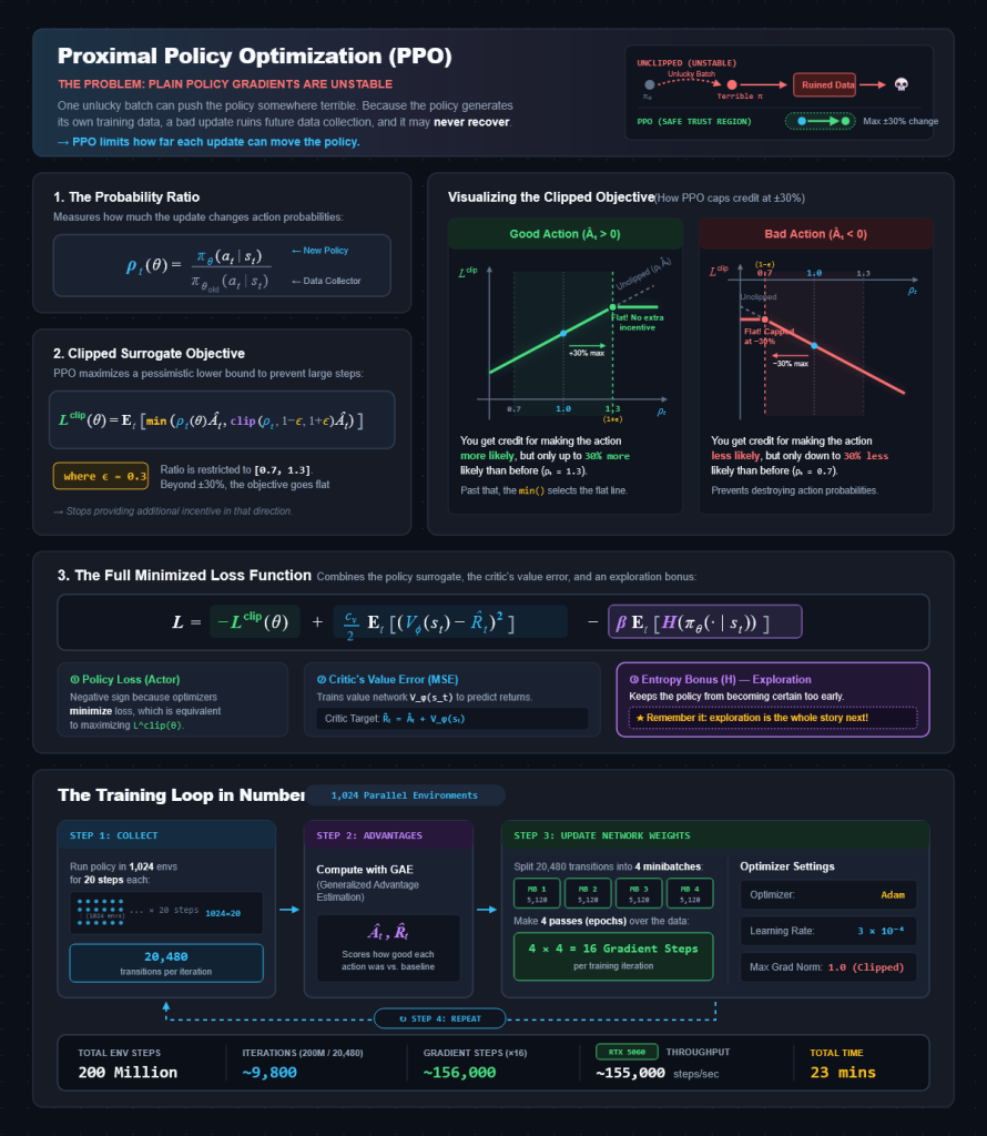
Define the probability ratio between the new policy and the one that collected the data: $\rho_t(\theta) = \frac{\pi_\theta(a_t \mid s_t)} {\pi_{\theta_{\text{old}}}(a_t \mid s_t)}$

PPO maximizes a clipped surrogate objective: $L^{\text{clip}}(\theta) = \mathbb{E}_t\left[ \min\left( \rho_t(\theta)\hat{A}_t,\; \operatorname{clip}\left( \rho_t(\theta), 1-\epsilon, 1+\epsilon \right)\hat{A}_t \right) \right]$

where $\epsilon = 0.3$ .

If an action was good ( $\hat{A}_t > 0$ ), you get credit for making it more likely, but only up to 30% more likely than before. If it was bad, you get credit for making it less likely, but only down to 30% less. Past that, the clipped objective stops providing additional incentive in that direction.

The full loss that’s minimized adds the critic’s error and an entropy bonus: $\begin{aligned} \mathcal{L} ={}& -L^{\text{clip}}(\theta) \\ &+ \frac{c_v}{2}\, \mathbb{E}_t\left[ \left(V_\phi(s_t)-\hat{R}_t\right)^2 \right] \\ &-\beta\,\mathbb{E}_t\left[ \mathcal{H}\left(\pi_\theta(\cdot \mid s_t)\right) \right] \end{aligned}$

where $\hat{R}_t = \hat{A}_t + V_\phi(s_t)$ is the critic’s training target and $\mathcal{H}$ is the policy’s entropy. The entropy term keeps the policy from becoming certain too early. Remember it, because exploration is the whole story of the next section.

The training loop in numbers

With 1024 parallel environments:

Collect: run the policy for 20 steps in all 1024 environments → 20,480 transitions
Compute advantages with GAE
Update. We split the data into 4 minibatches of 5,120 transitions and make 4 passes (epochs) over the data, giving 16 gradient steps in total. We use Adam with a learning rate of $3 \times 10^{-4}$ and clip gradients to a maximum norm of 1.0.
Repeat

200 million environment steps is about 9,800 iterations and 156,000 gradient steps. On the RTX 5060 this ran at ~155,000 environment steps per second: 23 minutes in total.

7. Case study: why the robot learned to stand still

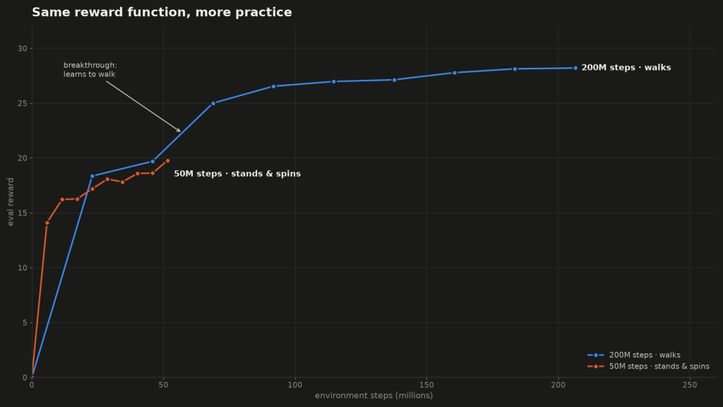
Here’s the failure. After 50 million steps, the evaluation reward had climbed to ~20 and was still slowly rising. It looked like progress. Then we measured what the robot actually did, holding each command fixed:

Command	Target	Achieved (50M steps)
forward	0.5 / 1.0 m/s	0.00
backward	0.5 m/s	0.00
sideways	0.4 m/s	0.00
turn	0.8 rad/s	0.62

Zero forward motion for every walk command. It had learned to stand perfectly still and turn in place. It never fell.

The math of the trap

Plug standing still into the reward. Say the command is “walk forward at 0.5 m/s,” and the robot stands still at its default pose: $r_{\text{lin}} = \exp\left(-\frac{0.5^2}{0.25}\right) = e^{-1} \approx 0.37$

Even though the robot is doing nothing, the Gaussian kernel still gives it 37% of the tracking reward. Then:

$r_{\text{yaw}} = 1$ : commanded turn rate is 0, actual turn rate is 0, so tracking is perfect.
$r_{\text{pose}} = 1$ : it’s exactly at the default pose, so the pose reward is perfect.

Weighted reward: $1.0(0.37) + 0.5(1) + 0.5(1) = 1.37$

That’s out of the roughly 2.0 available per step. Standing still banks about two-thirds of the positive reward.

Averaged over the training distribution of forward commands, $v_x^* \sim U(-1.5, 1.5)$ : $\mathbb{E}\left[e^{-v^2/\sigma}\right] = \frac{1}{3}\int_{-1.5}^{1.5} e^{-v^2/\sigma}\,dv$

With $\sigma = 0.25$ , this becomes $\frac{1}{3}\int_{-1.5}^{1.5} e^{-4v^2}\,dv = \frac{\sqrt{\pi}}{6}\operatorname{erf}(3) \approx 0.295$

So standing still collects about 30% of the forward-tracking reward on average, for free, plus full credit whenever the command happens to be zero.

And standing costs almost nothing. Look at the penalties: feet_clearance scales with foot speed (zero when feet are planted), feet_slip needs moving feet, energy and torques are minimal, action_rate is zero for constant actions, and stand_still only penalizes leaving the default pose.

Walking badly, meanwhile, is expensive. An early attempt at a step lifts a foot (clearance and height penalties), shifts weight (orientation penalty), moves joints away from the default pose (losing pose reward), and often ends in a fall (termination, plus all the future reward lost). The per-step reward is also clipped at zero, so a clumsy step can’t even be “worth” negative, and a fall throws away every future positive step.

So from the robot’s point of view there’s a valley between “stand still” and “walk well”. Standing is a solid local optimum. Moving a little away from it in any direction makes the reward worse. Only a coordinated gait, several joints moving together in a rhythm, is better. A policy-gradient method only follows the local slope, so it needs exploration noise to stumble across the far side of the valley.

Turning in place is the exception that proves the rule: rotating doesn’t require breaking the stance much, so the policy could improve yaw tracking in small, safe increments. That’s exactly the part it learned.

How it got out

We trained longer, with the identical setup: 1024 environments, 200 million steps instead of 50 million.

Steps	Eval reward
50M	~19
96M	20.7
106M	22.5
117M	25.3
200M	27.6

Between ~96M and ~117M steps, the reward jumped, and the robot started walking:

Command	Target	Achieved (200M steps)
forward	1.0 m/s	0.97
backward	0.5 m/s	0.47
sideways	0.4 m/s	0.36
turn	0.8 rad/s	0.75

Within ~10% on every command, and it never fell. A run with 8192 environments (upstream’s default) broke through earlier, at around 46–69M steps, but it ran about 4× slower per step on this GPU, so it took 96 minutes instead of 23.

Why the sudden jump instead of a smooth climb? We didn’t instrument this, so treat it as a hypothesis: the stochastic policy keeps sampling small leg movements around the standing pose. Eventually some of those samples line up into partial steps that beat standing for fast commands (where standing only earns $e^{-4} \approx 0.02$ of the tracking reward at 1 m/s). Once the advantage estimates start favoring stepping, PPO reinforces it quickly, and the gait improves itself.

The lesson

Reward going up is not the same as the task being learned. A reward of 20 looked like progress, and it meant “stand and spin”. The only way to see that was to test the behavior directly: hold each command fixed and measure the actual velocity. That evaluation is now part of every run.

8. Why the GPU matters: throughput math

PPO is sample-hungry, and this task needed more than 100 million steps just to get past the standing trap. That’s where GPU-batched simulation pays off.

Setup	Throughput	200M steps
1024 envs, RTX 5060	~155,000 steps/s	23 min
8192 envs, RTX 5060	24,000–47,000 steps/s	96 min

More parallel environments isn’t automatically faster. The 8192-environment run was slow, and it sped up as training went on. Our working hypothesis is the Warp contact solver: it reserves a fixed pool of contact slots shared across all environments (32,768, so ~4 per robot at 8192), and early in training, flailing robots generate many contacts. We haven’t verified that yet.

9. A teaser: the physics of a push

The real question in this series is robustness: does teaching the robot in stages (stand → balance → walk → survive pushes) make it better at recovering from shoves it’s never felt?

To measure that, we built a push test. It applies a horizontal force $F$ to the torso for a short time $\Delta t_p$ , from 8 directions, at random points in the gait. The impulse changes the robot’s momentum, so the velocity kick is $\Delta v = \frac{F\,\Delta t_p}{m}, \qquad m = 12.7\ \text{kg}$

Here, $m$ is the mass of the whole robot.

Our walking baseline, which never saw a push in training, handled this:

Push (100 ms)	$\Delta v$	Fell	Recovered
≤ 200 N	≤ 1.6 m/s	0%	100%
250 N	2.0 m/s	6%	94%
300 N	2.35 m/s	59%	41%
400 N	3.1 m/s	94%	6%

It handles pushes up to a point, then fails abruptly between $\Delta v \approx 2$ and 2.5m/s.

The environment also has its own training pushes: a half-sine force pulse, $F(t) = \frac{1}{2}\sin\left(\frac{\pi t}{T}\right) \cdot \frac{m v_{\text{kick}}}{T}$

Integrating it over the pulse gives the velocity change: $\Delta v = \frac{1}{m}\int_0^T F(t)\,dt$

Substituting the force profile: $\Delta v = \frac{v_{\text{kick}}}{2T} \int_0^T \sin\left(\frac{\pi t}{T}\right)\,dt$

Evaluating the integral: $\Delta v = \frac{v_{\text{kick}}}{2T} \cdot \frac{2T}{\pi} = \frac{v_{\text{kick}}}{\pi}$

With the default $v_{\text{kick}} \leq 3$ m/s, training pushes never exceed approximately ~0.95 m/s, far below the breaking point.

That gives us a clean setup: train with mild pushes, test with strong ones the robot has never felt, and compare direct training against a curriculum.

That’s Part 2.

Appendix: configuration

Setting	Value
Robot / task	Unitree Go1, `Go1JoystickFlatTerrain` (MuJoCo Playground)
Physics	MJX with Warp backend, 0.004 s timestep, 1 solver iteration
Control	50 Hz, PD joint targets, $K_p = 35$, $K_d = 0.5$, action scale 0.5
Episode	1000 steps (20 s)
Policy / value nets	MLP 512-256-128, swish; actor 48 inputs, critic 123
Action distribution	tanh-squashed Gaussian
PPO	$\gamma = 0.97$, $\lambda = 0.95$, $\epsilon = 0.3$, entropy 0.01, Adam lr $3 \times 10^{-4}$, grad clip 1.0
Batch	1024 envs × 20-step rollouts, 4 minibatches, 4 epochs
Budget	200M environment steps
Software	JAX 0.9.2, Brax 0.14.2, MuJoCo/MJX 3.17.0, Playground 0.2.0, Warp 1.18.0
Hardware	RTX 5060 8 GB, WSL2 Ubuntu 24.04