How KNN Actually Works

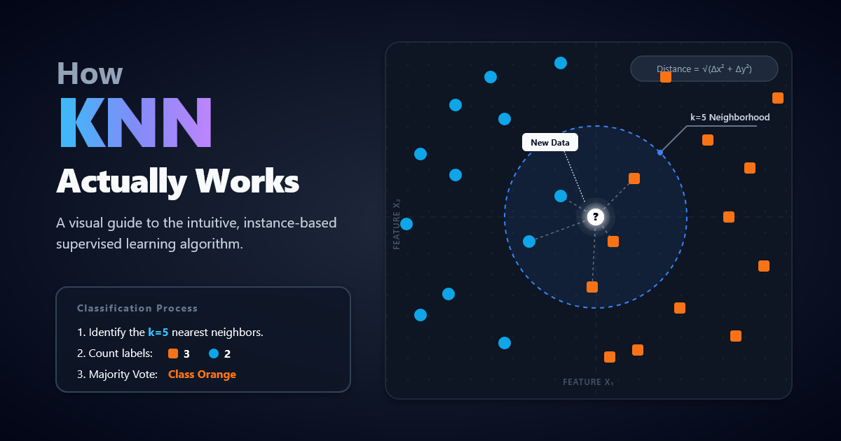
K-Nearest Neighbors, or KNN, is one of the most intuitive supervised learning methods: to predict a new point, it finds the k training examples that are closest under a chosen distance metric, then uses those neighbors to make the prediction. In classification, the prediction is usually a majority vote of nearby labels; in regression, it is usually the mean of nearby target values. KNN is non-parametric and instance-based: instead of learning one global equation, it stores examples and reasons locally at prediction time. That simplicity is its biggest strength—and also why metric choice, feature scaling, the value of k, and search efficiency matter so much. Larger k usually reduces noise but smooths away local detail; unscaled features can distort “closeness”; and brute-force search can be expensive, though KD-trees, ball trees, and approximate nearest neighbor indexes can help on the right kinds of data. [1]

What KNN is

Formally, KNN is a supervised learning family with two common flavors: classification for discrete labels and regression for continuous targets. Scikit-learn describes neighbors-based classification as an instance-based, non-generalizing method that stores training cases and predicts by majority vote among nearby points; for regression, the predicted value is computed from the mean of the nearest neighbors’ target values. IBM’s overview likewise describes KNN as a non-parametric supervised method that uses proximity to make classifications or predictions. [2]

A beginner-friendly analogy is this: if you want to decide whether a restaurant is “popular,” you ask the people standing closest to it. If most nearby people are entering, you call it popular. If you want to estimate a house price, you do something similar: look at the prices of the most similar nearby houses and average them. KNN works because it assumes that similar points tend to have similar outputs—but only if your notion of similarity is sensible. [3]

Suggested visual: a 2D scatter plot with x-axis = “study hours,” y-axis = “practice score,” blue circles = “pass,” red triangles = “fail,” and a black star = the new student. Draw dashed rings around the star until the 3 nearest points are enclosed; if 2 of the 3 are blue, KNN predicts “pass.” For regression, keep the same plot but replace class labels with numeric values like house prices, then average the neighbors’ values. See our KNN playground here.

Aspect	Summary
Pros	No global model must be fit first; KNN predicts directly from stored nearby examples, and nearest-neighbor classifiers can form highly irregular decision boundaries. [4]
Cons	Prediction can be costly, results are sensitive to scaling, metric, and k, and high-dimensional data can make nearest-neighbor search much less effective. [5]
Typical use-cases	Discrete-label classification, continuous-target regression, and similarity retrieval when “nearness” is meaningful and an appropriate metric or index is available. [6]

Walking through one prediction

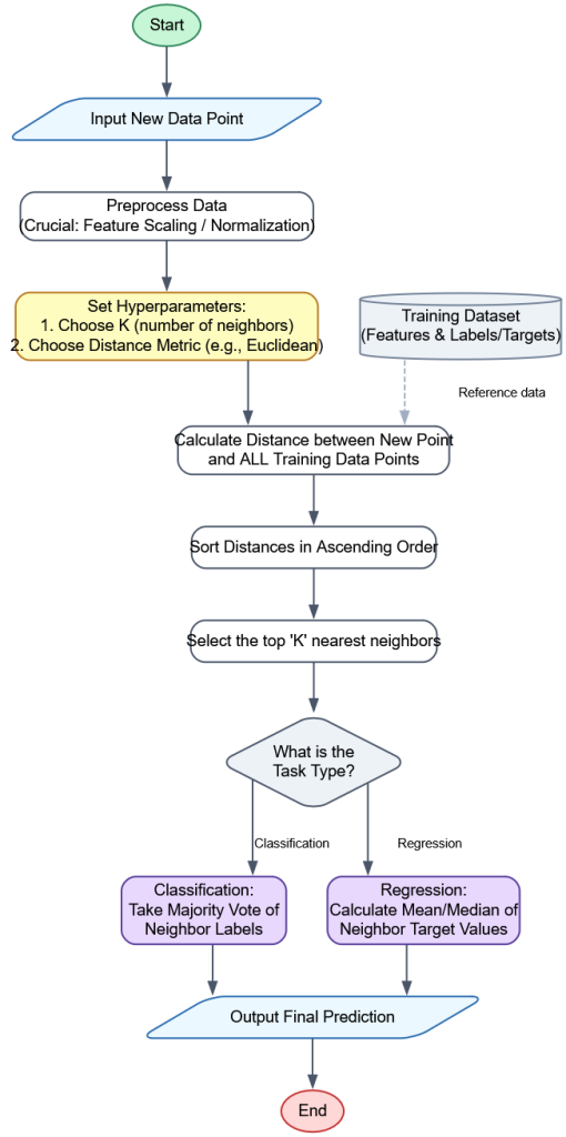
The core algorithm is short. First, keep the training set. Second, when a new query point arrives, compute its distance to every stored point—or use an index that finds the closest ones faster. Third, select the k nearest. Finally, aggregate their outputs: majority vote for classification, mean for regression. Scikit-learn also supports distance weighting, where closer neighbors count more than farther ones. [7]

Input: training data {(x_i, y_i)}, query q, k, distance d

for each training point x_i:
    compute distance d_i = d(q, x_i)

S = the k points with smallest d_i

if task is classification:
    return majority_label(S)
    # or distance-weighted vote
else:
    return mean(targets in S)
    # or distance-weighted mean

The important beginner insight is that KNN’s “training” is light because it mainly stores the data, while much of the real work happens at prediction time. That is why KNN often feels simple to fit but slower to deploy at scale. [8]

Choosing distance and neighborhood size

The distance metric controls what “similar” means. In scikit-learn, metric=’minkowski’ with p=2 gives Euclidean distance by default, and p=1 gives Manhattan distance. SciPy defines the common formulas directly. [9]

Metric	Formula	When it is a good beginner choice
Euclidean	d(x,y) = √∑(x_i – y_i)²	Default for continuous numeric features after scaling. It matches ordinary geometric distance.
Manhattan	d(x,y) = ∑\|x_i – y_i\|	Useful when you want coordinate-by-coordinate absolute differences rather than straight-line distance.
Minkowski	d(x,y) = (∑\|x_i – y_i\|^p)^1/p	A flexible family: p = 1 gives Manhattan, p = 2 gives Euclidean.
Cosine	d(x,y) = 1 – (x · y)/(\|x\|\|y\|)	Good when direction matters more than magnitude, such as normalized text or embedding vectors.

Choosing k is a bias-variance tradeoff. Scikit-learn’s neighbors guide notes that a larger k suppresses noise, but also makes class boundaries less distinct. In practice, choose k by validation or cross-validation rather than guesswork; scikit-learn even notes that knn.fit(X, y).score(None, y) is equivalent to leave-one-out cross-validation for KNN classification. An odd k can reduce ties in binary classification, but it does not guarantee safety: scikit-learn warns that if neighbor k and k+1 are at identical distances with different labels, the result can depend on training-data order. Distance weighting is often a practical fix because it gives nearer points more influence. [18]

Feature scaling is not optional for KNN on mixed-scale numeric data. Scikit-learn’s feature-scaling example explicitly shows that KNeighbors models can produce a completely different fit when data are unscaled, because distances become dominated by larger-range features. For categorical variables, vanilla KNN still needs a numeric representation: OneHotEncoder converts discrete strings or integers into binary columns, and scikit-learn’s valid metric lists include boolean-style distances such as Hamming and Jaccard for some neighbor-search back ends. A practical beginner rule is: one-hot encode nominal categories, then choose a metric that makes sense for binary indicators; do not invent fake numeric geometry with arbitrary label IDs. [19]

For complexity, brute-force neighbor search scales poorly: scikit-learn states that all-pairs brute force scales as ODN2, while query time grows as ODN. Tree-based methods can reduce search to roughly ODlogN in favorable settings, but KD-trees are most effective in lower dimensions—roughly fewer than 20—and can degrade toward brute force in higher dimensions. For very small datasets, brute force can even be faster than trees. [20]

Making KNN practical

If KNN is slow or brittle, the first lever is feature space. Scikit-learn’s Neighborhood Components Analysis section notes that NCA can learn a low-dimensional projection for visualization and faster classification, and its dimensionality-reduction examples compare 3-NN performance after projection into two dimensions. More broadly, reducing irrelevant or redundant dimensions can help because nearest-neighbor methods suffer from the curse of dimensionality. [21]

The second lever is indexing. Scikit-learn supports brute force, KD-tree, and ball tree search. KD-trees can be very efficient in lower-dimensional spaces; ball trees can outperform KD-trees in higher dimensions depending on the structure of the data. Scikit-learn also notes that precomputed neighbor graphs can come from custom estimators, including approximate nearest-neighbor methods. In practice, common external choices are Faiss, which targets efficient similarity search from millions to billions of dense vectors, and Annoy, which builds approximate nearest-neighbor indexes with small memory usage and memory-mapped read-only files. [22]

Here is a simple scikit-learn classification example. The StandardScaler is included because KNN is sensitive to scale. [23]

from sklearn.datasets import load_iris
from sklearn.model_selection import train_test_split
from sklearn.pipeline import make_pipeline
from sklearn.preprocessing import StandardScaler
from sklearn.neighbors import KNeighborsClassifier

X, y = load_iris(return_X_y=True)

X_train, X_test, y_train, y_test = train_test_split(
    X, y, test_size=0.25, stratify=y, random_state=42
)

model = make_pipeline(
    StandardScaler(),
    KNeighborsClassifier(n_neighbors=5, weights="distance")
)

model.fit(X_train, y_train)

print("Test accuracy:", model.score(X_test, y_test))
print("First 5 predictions:", model.predict(X_test[:5]))

Common pitfalls and beginner FAQs

Why does KNN sometimes look great in a notebook but disappoint in production? Because it postpones work until prediction. The method stores training examples, then must search neighborhoods for each new query; that is fine for small data, but expensive for large or latency-sensitive systems unless indexing or approximate search is added. [24]

Why did accuracy get worse after I added more features? More features do not automatically mean better neighborhoods. High-dimensional spaces make nearest-neighbor search less effective, which is one classic form of the curse of dimensionality. One-hot encoding can also increase dimensionality substantially because it creates a binary column per category. [25]

Should I always standardize features? For KNN, usually yes when numeric features are on different scales. If one feature spans a huge range and another spans a tiny one, the larger-scale feature can dominate the distance and change the model qualitatively. [26]

What is the beginner takeaway? KNN is best understood as “predict locally.” It works when local similarity is meaningful, your distance metric reflects the real problem, and your preprocessing preserves that geometry. If those choices are wrong, KNN fails for understandable reasons—which is exactly why it is such a good algorithm for learning the foundations of machine learning. [27]

Where should I read next? For readers who want a gentler textbook treatment after this post, the authors’ An Introduction to Statistical Learning family is explicitly designed as a broad, less technical introduction; for a deeper mathematical reference, The Elements of Statistical Learning is the classic next stop. [28]