
September 6, 2025
Multi-armed bandit problem; Your First Reinforcement Learning Agent in 100 Lines of C
Introduction
The landscape of modern machine learning education is dominated by Python. Its vast ecosystem of libraries like TensorFlow, PyTorch, and scikit-learn provides powerful abstractions that allow developers to build complex models with remarkable speed. While this is invaluable for productivity, it can also create a “black box” effect, where the fundamental mechanics of an algorithm are hidden behind a simple function call. To truly understand how an algorithm learns, adapts, and makes decisions, one must look under the hood. This requires moving beyond high-level abstractions and engaging with the code at a more foundational level.
This is where the C programming language offers a unique and powerful pedagogical advantage. By implementing algorithms in C, a developer is forced to confront the core logic directly. There are no libraries to abstract away memory management, no built in functions to find the maximum value in an array every component must be built from first principles. This process cultivates a deeper, more robust mental model of how the algorithm actually works, revealing its computational costs, memory footprint, and operational flow.
This is essentially the “Hello, World!” of Reinforcement Learning (RL): the Multi-Armed Bandit (MAB) problem. It is the simplest formulation of an RL task, stripping away the complexity of environments with multiple states to focus on the most fundamental challenge in decision making: the trade-off between exploring new options and exploiting known ones. This makes it the perfect starting point for our journey. The objective of this report is to guide the reader through the process of building, compiling, and running a complete RL agent in C. By the end, the reader will not only grasp the theory but will possess a tangible, working piece of C code that embodies a core principle of artificial intelligence.
The Gambler’s Dilemma: Deconstructing the Multi-Armed Bandit Problem
The Multi-Armed Bandit problem gets its name from a classic, intuitive analogy: a gambler in a casino facing a row of slot machines, colloquially known as “one-armed bandits”. Each machine has its own hidden, unique probability of paying out a reward. The gambler has a limited number of coins (or trials) and wants to walk away with the maximum possible winnings. The dilemma is clear: should the gambler stick with the machine that has paid out the most so far, or should they try other machines in the hope of finding one with an even better, yet undiscovered, payout rate?
Formalizing the Problem
This analogy can be translated into the formal language of reinforcement learning :
- Arms (K): The set of K available actions the agent can take. In our analogy, each slot machine is an “arm.”
- Rewards (R): At each time step, the agent chooses one arm to “pull.” This action, a, yields a reward, R, which is drawn from an unknown probability distribution specific to that arm.
- Objective: The agent’s goal is to devise a strategy, or policy, for choosing arms that maximizes the cumulative reward over a fixed number of trials, T.
The core challenge is that the reward distributions are unknown a priori. The agent can only learn about them by taking actions and observing the outcomes. This leads directly to the central conflict of the MAB problem.
The Exploration-Exploitation Trade-off
At the heart of the Multi-Armed Bandit problem lies the exploration-exploitation trade-off, a fundamental dilemma that extends far beyond RL into fields like economics, decision theory, and even natural selection.
- Exploitation: This is the strategy of using the knowledge the agent has already acquired to make the best decision right now. It involves choosing the action that currently has the highest estimated value—pulling the arm that has, on average, provided the best rewards so far.
- Exploration: This is the strategy of gathering new information. It involves choosing actions other than the current best, including those that have been tried infrequently or have performed poorly in the past. The goal is to improve the agent’s estimates of the arms’ true values, which could lead to better long-term rewards at the risk of a lower immediate payoff.
A simple, non-technical example illustrates this perfectly: choosing where to eat in a new city. On the first night, a person might find a restaurant that is quite good. For the rest of the trip, they face a choice. They can
exploit their knowledge by returning to that same restaurant, guaranteeing a good meal. Or, they can explore by trying a new, unknown restaurant. This new restaurant could be a disappointment, or it could be the best meal of their life. The agent cannot explore and exploit simultaneously; every decision to explore is a decision not to exploit, and vice versa. This is the essence of the dilemma the MAB agent must solve.
A Pragmatic Strategy: The Epsilon-Greedy Algorithm
The epsilon-greedy algorithm is one of the simplest and most widely used strategies for solving the MAB problem. It addresses the exploration-exploitation dilemma with a straightforward probabilistic rule.
The Core Logic
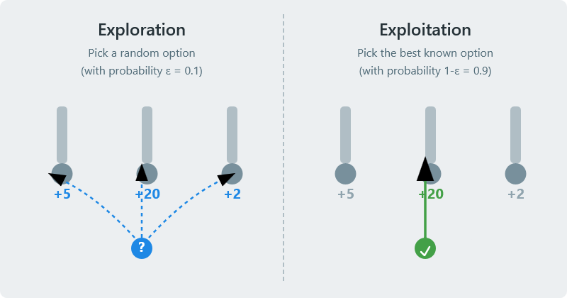
The algorithm’s behavior is governed by a single parameter, epsilon (ϵ), which represents the “exploration rate”. At each decision point, the agent acts as follows:
- With probability 1−ϵ, the agent exploits. It behaves “greedily” by selecting the action (arm) that it currently estimates to have the highest value.
- With probability ϵ, the agent explores. It ignores its current knowledge and selects an action at random from the set of all available actions, with each action having an equal chance of being chosen.
The epsilon parameter is typically a small value, for example, ϵ=0.1, which means the agent will explore 10% of the time and exploit the other 90%. Setting
ϵ too high results in excessive exploration, slowing down learning as the agent fails to capitalize on its knowledge. Conversely, setting it too low risks premature convergence, where the agent locks onto a suboptimal arm it discovered early on and never finds the true best option.
Action-Value Estimation
To make greedy choices, the agent needs a way to quantify its knowledge. This is done by maintaining an action-value estimate, denoted as Qt(a), for each arm a at time step t. This value represents the agent’s current best guess of the expected reward for pulling that arm.
The most common method for this is the sample-average method, where Qt(a) is simply the arithmetic mean of all rewards received from selecting arm a up to time step t-1.
The Incremental Update Rule
A naive implementation of the sample-average method would require storing a list of all rewards received for each arm and recalculating the average after every pull. This is inefficient in terms of both memory and computation. A much more elegant and efficient approach is to use an incremental update formula.
After the n-th time an arm is selected and a new reward Rn is received, its value estimate Qn can be updated to Qn+1 using the following rule:
Qn+1=Qn+n1(Rn−Qn)This formula can be interpreted intuitively as:
NewEstimate=OldEstimate+StepSize×(Target−OldEstimate)Here, the “Target” is the most recent reward Rn, and the “StepSize” is n1, which decreases as more samples are collected for that arm. This formula allows the agent to update its estimates using only the previous estimate, the new reward, and the number of times the arm has been pulled. This is a crucial optimization, as it reduces the memory requirement for each arm to a constant, regardless of the number of trials. This efficiency is particularly valuable in a C implementation, where memory management is explicit and avoiding dynamic array resizing leads to simpler and faster code.
Epsilon Decay
A common enhancement to the standard epsilon-greedy approach is to use epsilon decay. The agent starts with a high value of ϵ (e.g., 1.0, for pure exploration) and gradually reduces it over the course of the trials. This strategy is highly effective because it prioritizes exploration in the beginning when the agent’s knowledge is limited and shifts toward exploitation later on as its value estimates become more reliable.
From Pseudocode to Pointers: Implementing Epsilon Greedy in C
This section provides a detailed, line-by-line walkthrough of a complete epsilon-greedy agent implemented in C. This implementation reveals the underlying machinery that is often concealed by higher-level languages.
The Setup: Headers and Constants
The program begins by including the necessary standard libraries and defining key parameters for the simulation.
#include <stdio.h>
#include <stdlib.h>
#include <time.h>

// --- Configuration ---
#define NUM_ARMS 5
#define NUM_TRIALS 10000
#define EPSILON 0.1<stdio.h>is included for standard input/output functions, primarilyprintf.<stdlib.h>provides functions for memory allocation (malloc), pseudo-random number generation (rand,srand), and string conversion.<time.h>is used to seed the random number generator to ensure different outcomes on each run.- Using
#definefor configuration parameters likeNUM_ARMS,NUM_TRIALS, andEPSILONmakes the code easy to read and modify for different experiments.
Data Structures: The Agent’s Memory
The agent’s “brain” its memory of each arm’s performance is captured in a simple struct.
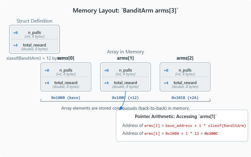
// Represents a single arm of the bandit
struct BanditArm {
    double estimated_value;
    int times_pulled;
};
estimated_value: This corresponds to Q(a), the current estimated average reward for this arm.times_pulled: This is the count, n, of how many times this arm has been selected. This is needed for the incremental update rule.
Core Functions
The logic of the agent is broken down into several small, focused functions.
argmax: Finding the Best Action
Unlike Python’s NumPy, C does not have a built-in argmax function to find the index of the maximum value in an array. It must be implemented manually.
// Find the index of the arm with the highest estimated value
int argmax(struct BanditArm* arms, int n_arms) {
    int best_arm = 0;
    double max_value = arms[0].estimated_value;
    for (int i = 1; i < n_arms; i++) {
        if (arms[i].estimated_value > max_value) {
            max_value = arms[i].estimated_value;
            best_arm = i;
        }
    }
    return best_arm;
}
This function iterates through the array of BanditArm structs, keeping track of the highest estimated_value seen so far and the index at which it was found. For simplicity, it breaks ties by returning the index of the first maximum value encountered.
select_action: The Heart of the Algorithm
This function implements the core epsilon-greedy decision logic.
// Select an action using the epsilon-greedy strategy
int select_action(struct BanditArm* arms, int n_arms, double epsilon) {
    // Generate a random number between 0.0 and 1.0
    double rand_val = (double)rand() / RAND_MAX;

    if (rand_val < epsilon) {
        // Exploration: choose a random arm
        return rand() % n_arms;
    } else {
        // Exploitation: choose the best known arm
        return argmax(arms, n_arms);
    }
}
- A random floating-point number is generated by casting the integer output of
rand()to adoubleand dividing byRAND_MAX, the maximum valuerand()can return. - This value is compared to
epsilon. If it’s smaller, the agent explores by returning a random arm index (rand() % n_arms). - Otherwise, the agent exploits by calling the
argmaxfunction to find and return the index of the best-performing arm.
get_reward: Simulating the Environment
To test the agent, a function is needed to simulate pulling an arm and receiving a reward. This function models a Bernoulli distribution: it returns a reward of 1.0 with a given probability (the “win rate”) and 0.0 otherwise.
// Simulate pulling an arm and getting a reward (1 for win, 0 for loss)
double get_reward(double true_payout_prob) {
    double rand_val = (double)rand() / RAND_MAX;
    return (rand_val < true_payout_prob)? 1.0 : 0.0;
}
update_estimate: Implementing the Learning Rule
This function applies the incremental update formula to adjust the agent’s knowledge after receiving a reward.
// Update the arm's estimated value using the incremental update rule
void update_estimate(struct BanditArm* arm, double reward) {
    arm->times_pulled++;
    double step_size = 1.0 / arm->times_pulled;
    arm->estimated_value += step_size * (reward - arm->estimated_value);
}
This is a direct C implementation of the formula Qn+1=Qn+n1(Rn−Qn).
The main() Function: Orchestrating the Simulation
The main function initializes the environment and the agent, then runs the simulation loop.
int main() {
    // Seed the random number generator for different results on each run
    srand((unsigned)time(NULL));

    // Make true payouts an array
    const double true_payouts[NUM_ARMS] = {0.2, 0.5, 0.75, 0.4, 0.6};

    // Make arms an array
    struct BanditArm arms[NUM_ARMS];
    for (int i = 0; i < NUM_ARMS; i++) {
        arms[i].estimated_value = 0.0;
        arms[i].times_pulled = 0;
    }

    double total_reward = 0.0;

    // Main simulation loop
    for (int trial = 0; trial < NUM_TRIALS; trial++) {
        // 1. Select an action
        int chosen_arm = select_action(arms, NUM_ARMS, EPSILON);

        // 2. Get a reward from the environment
        double reward = get_reward(true_payouts[chosen_arm]);

        // 3. Update the agent's knowledge
        update_estimate(&arms[chosen_arm], reward);

        // 4. Accumulate total reward
        total_reward += reward;
    }

    // --- Print final results ---
    printf("Simulation finished after %d trials.\n", NUM_TRIALS);
    printf("Total reward accumulated: %.2f\n", total_reward);
    printf("Overall average reward: %.4f\n\n", total_reward / NUM_TRIALS);

    printf("Final estimated values vs. true values:\n");
    int best_arm_true = 0;
    for(int i = 1; i < NUM_ARMS; i++) {
        if (true_payouts[i] > true_payouts[best_arm_true]) {
            best_arm_true = i;
        }
    }

    for (int i = 0; i < NUM_ARMS; i++) {
        printf("Arm %d: Estimated Value = %.4f, True Value = %.4f, Times Pulled = %d",
               i, arms[i].estimated_value, true_payouts[i], arms[i].times_pulled);
        if (i == best_arm_true) {
            printf(" (OPTIMAL)");
        }
        printf("\n");
    }

    return 0;
}
srand(time(0)): This is a critical step. It seeds the pseudo-random number generator with the current system time, ensuring that the sequence of “random” numbers is different each time the program is executed.- The
true_payoutsarray represents the ground truth of the environment, which the agent must discover. - The main loop executes the core RL cycle: select an action, get a reward, and update the estimate.
- Finally, the program prints a summary of the results, comparing the agent’s learned estimates to the true payout probabilities. This allows for a quick verification of whether the agent successfully identified the optimal arm.
The Complete Code (bandit.c)
#include <stdio.h>
#include <stdlib.h>
#include <time.h>
// --- Configuration ---
#define NUM_ARMS 5
#define NUM_TRIALS 10000
#define EPSILON 0.1
// Represents a single arm of the bandit
struct BanditArm {
double estimated_value;
int times_pulled;
};
// Find the index of the arm with the highest estimated value
int argmax(struct BanditArm* arms, int n_arms) {
int best_arm = 0;
double max_value = arms.estimated_value;
for (int i = 1; i < n_arms; i++) {
if (arms[i].estimated_value > max_value) {
max_value = arms[i].estimated_value;
best_arm = i;
}
}
return best_arm;
}
// Select an action using the epsilon-greedy strategy
int select_action(struct BanditArm* arms, int n_arms, double epsilon) {
// Generate a random number between 0.0 and 1.0
double rand_val = (double)rand() / RAND_MAX;
if (rand_val < epsilon) {
// Exploration: choose a random arm
return rand() % n_arms;
} else {
// Exploitation: choose the best known arm
return argmax(arms, n_arms);
}
}
// Simulate pulling an arm and getting a reward (1 for win, 0 for loss)
double get_reward(double true_payout_prob) {
double rand_val = (double)rand() / RAND_MAX;
return (rand_val < true_payout_prob)? 1.0 : 0.0;
}
// Update the arm's estimated value using the incremental update rule
void update_estimate(struct BanditArm* arm, double reward) {
arm->times_pulled++;
double step_size = 1.0 / arm->times_pulled;
arm->estimated_value += step_size * (reward - arm->estimated_value);
}
int main() {
// Seed the random number generator for different results on each run
srand(time(0));
// Define the "true" payout probabilities for each arm (unknown to the agent)
double true_payouts = {0.2, 0.5, 0.75, 0.4, 0.6};
// Initialize the bandit arms
struct BanditArm arms;
for (int i = 0; i < NUM_ARMS; i++) {
arms[i].estimated_value = 0.0;
arms[i].times_pulled = 0;
}
double total_reward = 0.0;
// Main simulation loop
for (int trial = 0; trial < NUM_TRIALS; trial++) {
// 1. Select an action
int chosen_arm = select_action(arms, NUM_ARMS, EPSILON);
// 2. Get a reward from the environment
double reward = get_reward(true_payouts[chosen_arm]);
// 3. Update the agent's knowledge
update_estimate(&arms[chosen_arm], reward);
// 4. Accumulate total reward
total_reward += reward;
}
// --- Print final results ---
printf("Simulation finished after %d trials.\n", NUM_TRIA LS);
printf("Total reward accumulated: %.2f\n", total_reward);
printf("Overall average reward: %.4f\n", total_reward / NUM_TRIALS);
printf("\nFinal estimated values vs. true values:\n");
int best_arm_true = 0;
for(int i = 1; i < NUM_ARMS; i++) {
if (true_payouts[i] > true_payouts[best_arm_true]) {
best_arm_true = i;
}
}
for (int i = 0; i < NUM_ARMS; i++) {
printf("Arm %d: Estimated Value = %.4f, True Value = %.4f, Times Pulled = %d",
i, arms[i].estimated_value, true_payouts[i], arms[i].times_pulled);
if (i == best_arm_true) {
printf(" (OPTIMAL)");
}
printf("\n");
}
return 0;
}
Bringing Your Agent to Life: Compilation and Execution
With the source code complete, the next step is to compile it into an executable program and run it.
Prerequisites
A C compiler is required. The GNU Compiler Collection (GCC) is the standard for Linux and macOS and is easily installed on Windows via environments like MinGW or the Windows Subsystem for Linux (WSL).
Compilation
Open a terminal or command prompt, navigate to the directory where bandit.c is saved, and execute the following command :
gcc -Wall -o bandit bandit.c
Let’s break down this command:
gcc: Invokes the GCC compiler.-Wall: This is a highly recommended flag that enablesallcompilerwarning messages. It helps catch potential bugs and encourages writing cleaner code.-o bandit: This flag specifies the name of theoutput file. Without it, the compiler would default toa.out.bandit.c: This is the input source file.
Execution
Once the code compiles without errors, an executable file named bandit (or bandit.exe on Windows) will be created in the directory. To run it, use the following command :
./bandit
Interpreting the Output
The program will run the simulation and print a summary of the results. A typical output might look like this:
Simulation finished after 10000 trials.
Total reward accumulated: 7235.00
Overall average reward: 0.7235

Final estimated values vs. true values:
Arm 0: Estimated Value = 0.2238, True Value = 0.2000, Times Pulled = 210
Arm 1: Estimated Value = 0.5318, True Value = 0.5000, Times Pulled = 220
Arm 2: Estimated Value = 0.7521, True Value = 0.7500, Times Pulled = 9119 (OPTIMAL)
Arm 3: Estimated Value = 0.3198, True Value = 0.4000, Times Pulled = 197
Arm 4: Estimated Value = 0.5906, True Value = 0.6000, Times Pulled = 254
This output shows that the agent successfully learned. Its estimated values are very close to the true payout probabilities, and it correctly identified Arm 2 as the optimal choice, pulling it far more often than any other arm. The overall average reward of 0.7352 is very close to the maximum possible reward of 0.75, indicating a highly effective strategy.
Visualizing Success: Plotting Your Agent’s Learning Curve with Gnuplot
While the final printout is informative, a visual representation of the agent’s learning process provides a much more powerful and intuitive understanding of its performance. A plot of the average reward over time can clearly show whether the agent is improving its strategy.
This can be achieved by adopting a modular workflow common in scientific and systems programming: the C program will be responsible for computation and data generation, and a separate, specialized tool—Gnuplot—will handle the visualization. This separation of concerns is a robust design pattern that avoids bloating the C code with complex plotting library dependencies.
Modifying the C Code for Data Output
First, the C program must be modified to write its progress to a data file.
- At the beginning of the
mainfunction, open a file for writing:CFILE *f = fopen("results.dat", "w"); if (f == NULL) { printf("Error opening file!\n"); return 1; } - Inside the main simulation loop, after
total_rewardis updated, write the current trial number and the cumulative average reward to the file:Cfprintf(f, "%d %f\n", trial, total_reward / (trial + 1)); - At the end of the
mainfunction, beforereturn 0, close the file:Cfclose(f);
Introducing Gnuplot
Gnuplot is a powerful, command-line-driven graphing utility that has been a staple in scientific computing for decades. It excels at creating publication-quality plots from data files and can be controlled via simple scripts, making it a perfect companion for our C program.
Name        Length
----        ------
results.dat 148894
1 0.000000
2 0.000000
3 0.333333
4 0.250000
5 0.400000
The Gnuplot Script
Create a new text file named plot.gp and add the following commands:
Code snippet
# Set the output format and size
set terminal pngcairo size 800,600 enhanced font 'Verdana,10'
set output 'learning_curve.png'

# Set plot titles and labels
set title "Epsilon-Greedy Learning Curve (ε = 0.1)"
set xlabel "Trials"
set ylabel "Average Reward per Trial"
set grid

# Plot the data from our file
# 'using 1:2' means use column 1 for x-axis and column 2 for y-axis
plot 'results.dat' using 1:2 with lines title 'Agent Performance'
Generating the Plot
After recompiling and running the modified C program to generate results.dat, execute the following command in the terminal:
gnuplot plot.gp
This will read the script and generate a file named learning_curve.png. The resulting plot will show a curve that starts low and erratically but quickly rises and stabilizes near the optimal reward value, providing clear visual evidence of the agent’s learning process.
The Road Ahead: Next Steps in Your C-based RL Journey
The epsilon-greedy algorithm is a fantastic starting point due to its simplicity and effectiveness. However, it is not without its limitations. Its primary drawback is that its exploration is “naive”—when it decides to explore, it chooses a non-greedy action uniformly at random. This means it is just as likely to pick an arm it knows is terrible as it is to pick a promising but uncertain one.
More advanced algorithms address this by incorporating the concept of uncertainty into the action selection process, leading to more intelligent exploration.
A Comparison of Bandit Strategies
The following table provides a high-level comparison of epsilon-greedy with two popular and more sophisticated alternatives, offering a roadmap for future projects.
| Strategy | Core Idea | Pros | Cons |
| Epsilon-Greedy | With probability ϵ, explore randomly; otherwise, exploit the best-known arm. | Simple to implement, computationally cheap, guaranteed to eventually find the optimal arm. | Explores inefficiently (can pick known bad arms), performance is sensitive to the choice of ϵ. |
| Upper Confidence Bound (UCB) | “Optimism in the face of uncertainty.” Prefers arms with a high estimated value AND high uncertainty (i.e., arms that haven’t been tried often). | Explores more intelligently by prioritizing less-known arms, often converges faster than ϵ-greedy, has no hyperparameters like ϵ to tune. | More complex to implement, can perform poorly if reward variances are high or misspecified. |
| Thompson Sampling | A Bayesian approach. Models reward probabilities as distributions (e.g., Beta distributions) and samples from them to choose an action. | Very effective in practice, often outperforming UCB. Naturally balances exploration and exploitation based on posterior probabilities. | Conceptually more complex (requires understanding of probability distributions), can be computationally more intensive. |
From Bandits to Worlds: A Deep Dive into Q-Learning
The Multi-Armed Bandit is a special case of a Reinforcement Learning problem—one with only a single state. The next logical step is to explore environments where the agent’s actions can change its state, and the optimal action depends on the state it is in. This is the domain of algorithms like Q-learning. The next tutorial in this series will tackle this challenge, showing how to implement a Q-learning agent in C to solve a classic Gridworld problem, where an agent must learn the shortest path through a maze to a goal.
Conclusion
This report has detailed the journey of building a reinforcement learning agent from the ground up using the C programming language. It began with the foundational Multi-Armed Bandit problem, establishing the critical trade-off between exploration and exploitation that lies at the heart of decision-making under uncertainty. The epsilon-greedy algorithm was presented as a simple and effective strategy to balance this trade-off.
The core of the tutorial was a deep dive into a complete C implementation, demonstrating how to manage the agent’s state, implement the decision-making logic, and apply the incremental learning rule. By manually coding components like argmax and managing data structures directly, a level of understanding is achieved that is often obscured by the high-level libraries of other languages. Furthermore, the process of compiling the code, running the simulation, and visualizing the results with Gnuplot teaches a robust and practical workflow for computational experiments.
The reader has not just learned about an algorithm; they have built it. This hands-on experience provides a solid foundation for tackling more complex challenges in reinforcement learning. The path forward involves experimenting with the current code—tuning EPSILON, changing the number of arms, or altering the reward structures—and attempting to implement the more advanced bandit algorithms discussed. The principles learned here are directly applicable to the more general and powerful algorithms, such as Q-learning, that await on the horizon.