Why Your PyTorch Model Is Slower Than You Think (Even on GPU)

Tested on: RTX 5060 · PyTorch 2.7 · CUDA 13.1 · Windows 11

---

You moved your model to GPU. You watched nvidia-smi climb toward 100%. You assumed you were done.

You probably aren’t.

GPU utilization is a coarse, 100ms-sampled metric. A GPU can report 80% utilization while spending most of that time idle between kernels, starved by a DataLoader that can’t keep up, or stalled waiting for your Python code to read a loss value.

We’ll cover three categories of hidden bottlenecks I measured on a real RTX 5060 training loop. None of them are in your model architecture. All of them are fixable in minutes. And the numbers will probably surprise you, both in where the speedup is large, and where it isn’t.

---

The mental model you need first

Before the benchmarks, one concept: the CPU and GPU are two separate workers running in parallel.

When you call loss.backward(), PyTorch doesn’t wait for the GPU to finish. It queues work onto the CUDA stream and returns immediately. The CPU races ahead to the next line of Python while the GPU drains its work queue independently.

CPU:  [queue forward] [queue backward] [queue optimizer] [queue forward] ...
GPU:                  [  forward  ][   backward   ][ optimizer ][  forward  ] ...

This asynchrony is why GPUs are fast. The CPU is always preparing the next batch of work while the GPU executes the current one.

A synchronization point is anything that breaks this pipeline, forcing the CPU to stop and wait until the GPU finishes all pending work. The GPU goes idle. The CPU goes idle. Then they both start again from scratch.

This is the bubble. It’s invisible unless you’re looking for it.

---

Bottleneck 1: CPU → GPU sync points

The .item() tax — less than you’d expect

The most commonly cited sync point is .item(), which pulls a scalar value from the GPU to Python. Every tutorial warns about it. Most of the warnings are overstated.

Here’s what it actually costs on a compute-heavy model:

# Version A: .item() every step
running_loss += loss.item()   # sync on every iteration

# Version B: accumulate on GPU, read once
running_loss += loss.detach() # stays on GPU
total = running_loss.item()   # one sync at the end

Results (RTX 5060, 1024→2048→10 MLP, batch 256):

	ms/step
.item() every step	2.33ms
deferred .item()	2.26ms
Speedup	1.03x

3% faster. On this model, not worth losing sleep over.

Why? The GPU is doing 2ms of real computation per step. The sync overhead (0.1ms) is small relative to that. By the time Python calls .item(), the GPU has often already finished. There’s nothing to wait for.

The honest answer: a single .item() per step barely matters on modern hardware when your GPU kernels take several milliseconds.

The logging anti-pattern — where it actually hurts

Now here’s the version that actually bites people. A typical training loop with naive logging:

# What "just add some logging" looks like in practice
for step, (x, y) in enumerate(loader):
    optimizer.zero_grad()
    logits = model(x)
    loss = criterion(logits, y)
    loss.backward()
    optimizer.step()

    # Each of these is a separate sync point:
    log("loss", loss.item())                                    # sync 1
    log("accuracy", (logits.argmax(1) == y).float().mean().item())  # sync 2
    log("confidence", logits.max(dim=1).values.mean().item())   # sync 3
    log("logit_var", logits.var().item())                       # sync 4
    for p in model.parameters():
        log("grad_norm", p.grad.norm().item())                  # sync 5..N

Every .item() call is a full GPU stall. Six metrics logged naively means six sync points per step. Here’s what that looks like in the profiler:

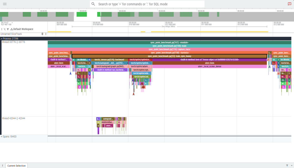
One complete train_sync_heavy step (~2.7ms) on the CPU training thread. The brown aten::item bars and the wide magenta aten::local_scalar_dense block (spanning roughly 60% of the step) are CPU stalls — every call forces the CPU to halt until the GPU drains its queue. There are 13 aten::item events per step, arriving in ~6 distinct synchronization clusters. The dominant stall at the right edge of the step is a single ~1.6ms block where the CPU is doing nothing but waiting.

The fix: keep everything on GPU until you’re done with the step, then move it all to CPU in a single operation.

    # Compute all metrics as GPU tensors — no syncs yet
    loss_t   = loss.detach()
    acc_t    = (logits.detach().argmax(1) == y).float().mean()
    conf_t   = logits.detach().max(dim=1).values.mean()
    var_t    = logits.detach().var()
    gnorm_t  = torch.stack([p.grad.norm()
                            for p in model.parameters()
                            if p.grad is not None]).mean()

    # Single sync: ship all scalars to CPU at once
    loss_v, acc_v, conf_v, var_v, gnorm_v = (
        torch.stack([loss_t, acc_t, conf_t, var_t, gnorm_t]).tolist()
    )

Here’s the same step after the fix, at the same zoom level:

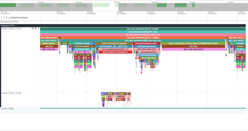
One complete train_sync_clean step at identical zoom. The 12 aten::item calls that were stalling the CPU now complete in 1–3 µs each — the GPU had already finished those ops asynchronously, so there was nothing to wait for. The single remaining aten::local_scalar_dense block at the far right is the one intentional sync: the final .item() call that moves the accumulated loss to Python. The step is the same duration, but the GPU was busy the whole time instead of repeatedly going idle.

Results (same model, same hardware):

	ms/step
Naive logging (N syncs/step)	3.06ms
Batched logging (1 sync/step)	2.40ms
Speedup	1.28x

27% slower. Just from how you read your metrics.

At 50,000 training steps, that’s the difference between a 2.5-hour run and a 3.2-hour run — for code that produces identical results.

The two culprits you won’t see in your own code

W&B and TensorBoard. Both call .item() internally when you pass a tensor to their logging APIs. If you’re calling wandb.log({"loss": loss}) inside your training loop, you have a sync point on every step. Pass a Python float instead: wandb.log({"loss": loss.item()}) — yes, the sync still happens, but now it’s your explicit choice and you can batch it.

Conditional branches on tensor values. This one is subtle:

if loss > threshold:          # forces .item() implicitly — Python must
    trigger_early_stop()      # know the value to evaluate the condition

Use torch.where or move threshold logic to a scheduled check every N steps instead.

How to find sync points in your own code

Run your training loop under torch.profiler with with_stack=True:

from torch.profiler import profile, ProfilerActivity, schedule, tensorboard_trace_handler

with profile(
    activities=[ProfilerActivity.CPU, ProfilerActivity.CUDA],
    schedule=schedule(wait=1, warmup=2, active=10),
    on_trace_ready=tensorboard_trace_handler("./traces"),
    with_stack=True,
) as prof:
    for step in range(13):
        train_step()
        prof.step()

Open the trace in Perfetto UI. Look for cudaStreamSynchronize events on the CPU thread. Each one is a sync point. The with_stack=True flag tells you exactly which Python line triggered it.

---

Bottleneck 2: DataLoader stalls

This is the one most likely to be destroying your throughput right now.

What starvation looks like

The DataLoader and the GPU training loop are a producer-consumer pipeline. The DataLoader produces batches; the GPU consumes them. When the producer is slower than the consumer, the GPU sits idle at the start of every step, waiting for data.

Open any profiler trace on a starved DataLoader and you’ll see it immediately: a long gap at the beginning of each training step, before a single GPU kernel has fired. The CPU is in DataLoader.__next__, doing PIL decodes and transforms in the main process, while the GPU is doing nothing.

The fix requires exactly two DataLoader arguments.

The num_workers sweep

DataLoader(dataset, batch_size=128, num_workers=N, pin_memory=True)

I measured throughput across 5 configs on a dataset with heavy image transforms (random crop, color jitter, normalize) at 224×224:

num_workers	pin_memory	samples/sec	speedup
0	False	505	1.0x
2	False	886	1.75x
2	True	957	1.9x
4	True	1,619	3.2x
8	True	2,281	4.52x

4.52x throughput improvement. Two arguments. The model, optimizer, and loss function are identical. The only change is how data gets to the GPU.

What these arguments actually do

num_workers=N spawns N worker processes that prefetch and transform batches in parallel. While the GPU is training on batch K, workers are already preparing batches K+1, K+2, … K+N. The GPU never waits.

num_workers=0 means the main process does all of this serially — fetch, transform, train, fetch, transform, train. The GPU is idle during every fetch+transform phase.

A reasonable starting value is num_workers = min(os.cpu_count(), 8). The throughput curve flattens or dips past a certain point (usually when worker processes start competing for memory bandwidth), so sweep a few values and pick the knee.

pin_memory=True allocates host tensors in page-locked memory. This lets the CUDA DMA engine transfer data to the GPU without CPU involvement, and — critically — allows that transfer to overlap with GPU compute on the previous batch. Without pinned memory, host→device transfers block on pageable memory and can’t be pipelined.

pin_memory=True only does anything useful when num_workers > 0. Workers must be the ones allocating the tensors for them to be pinned correctly. With num_workers=0, this flag is a no-op.

Windows-specific gotcha

On Windows, DataLoader workers use the spawn start method (not fork like Linux/macOS). This means:

1. Always wrap your training code in if __name__ == "__main__":. Without it, worker processes re-import your script, hit the training code again, try to spawn more workers, and crash or silently fall back to num_workers=0.
2. Worker startup overhead is higher on Windows than Linux. If you’re running short experiments (few batches per epoch), use persistent_workers=True to keep workers alive between epochs rather than paying the spawn cost every epoch.

One more option: persistent_workers=True

For workflows with many small epochs — hyperparameter sweeps, few-shot learning, anything where epochs are short — DataLoader workers are created and destroyed every epoch by default. On Windows with spawn, this has non-trivial overhead.

DataLoader(dataset, num_workers=4, pin_memory=True, persistent_workers=True)

Workers stay alive between epochs. The prefetch queue stays warm. First batch of each epoch arrives immediately instead of waiting for worker initialization.

---

Bottleneck 3: kernel launch overhead

What “small kernels” means

Every CUDA operation — a matrix multiply, an elementwise add, a layer norm — is a kernel: a program that runs on the GPU. Launching a kernel has a fixed CPU-side cost of roughly 5–20 microseconds, regardless of how much work the kernel does.

For a large matrix multiply that takes 5ms to execute, 20μs of launch overhead is noise. For a x = x + shift on a small tensor that takes 50μs to execute, 20μs of launch overhead is 40% of the total time for that operation.

A custom activation function written as sequential PyTorch ops — each line a separate kernel — stacks this overhead for every op, every layer, every step:

def forward(self, x):
    x = x * self.scale        # kernel 1
    x = x + self.shift        # kernel 2
    x = x - x.mean(...)       # kernels 3-4
    std = x.var(...).sqrt()   # kernels 5-7
    x = x / std               # kernel 8
    x = x * 0.5 * (1.0 + torch.tanh(...))  # kernels 9-15
    x = x.clamp(-10.0, 10.0)  # kernel 16
    return x

That’s 16 kernel launches per block, per layer, per step.

How much does it actually cost?

Here I’ll be honest with you: on a training-scale workload, probably not that much.

I benchmarked the above fragmented model (8 layers, batch 128, sequence length 64, dim 256) against torch.compile with the cudagraphs backend, which captures the entire kernel sequence and replays it as a single cudaGraphLaunch:

	ms/step
Eager (N kernel launches/step)	14.63ms
cudagraphs (1 launch/step)	13.83ms
Overhead	~5%

5%. On this model, GPU arithmetic dominates. The ~0.8ms of launch overhead is real but not catastrophic.

The picture changes significantly in two scenarios:

1. Inference with small batches. At batch size 1 for real-time inference, GPU kernels may complete in tens of microseconds. Launch overhead becomes a large fraction of total latency. This is where torch.compile routinely shows 2–4x speedups in the PyTorch benchmarks.

2. Many custom elementwise ops on small tensors. If you’ve written a custom loss function, regularizer, or activation with many sequential ops on small feature maps, the launch overhead compounds. The fix isn’t just torch.compile — check whether a fused implementation already exists in the ecosystem (Flash Attention, torch.nn.functional.scaled_dot_product_attention).

torch.compile on Windows

The default torch.compile backend (inductor) requires Triton, which has no official Windows support as of PyTorch 2.7. Use the cudagraphs backend instead:

model = torch.compile(model, backend="cudagraphs")

cudagraphs requires static input shapes — your batch size and sequence length must be fixed across steps. If you have variable-length sequences, pad to a fixed length or use torch.compile(model, dynamic=True) with the inductor backend on Linux.

One critical benchmarking note: the first several iterations of a compiled model are graph capture, not inference. They will be 10–100x slower than steady state. Always warm up for at least 10–15 steps before measuring, and never include iteration 1 in your numbers.

# Wrong: first iter is graph capture, not representative
t0 = time.perf_counter()
for i in range(100):
    run_step()
print((time.perf_counter() - t0) / 100)

# Right: warm up first
for _ in range(15):
    run_step()               # graph capture happens here
torch.cuda.synchronize()
t0 = time.perf_counter()
for _ in range(100):
    run_step()               # now measuring steady-state
torch.cuda.synchronize()
print((time.perf_counter() - t0) / 100)

---

Putting it together: how to actually profile your own code

The benchmark scripts for everything in this article are in the companion repo. But your model isn’t the same as mine. Here’s how to find your bottleneck.

Step 1: check GPU utilization

nvidia-smi dmon -s u -d 1

If utilization is consistently above 85%, your GPU is not the bottleneck — go look at your CPU code. If it’s low, continue.

Step 2: profile one training step

from torch.profiler import profile, ProfilerActivity, schedule, tensorboard_trace_handler

with profile(
    activities=[ProfilerActivity.CPU, ProfilerActivity.CUDA],
    schedule=schedule(skip_first=5, wait=1, warmup=2, active=5),
    on_trace_ready=tensorboard_trace_handler("./my_trace"),
    record_shapes=True,
    with_stack=True,
) as prof:
    for step in range(13):
        train_step(batch)
        prof.step()

The skip_first=5 skips early iterations where JIT compilation and DataLoader warmup pollute the trace. Always skip.

Step 3: read the trace

Open ./my_trace in Perfetto UI.

Look for these three patterns in order:

Gap at the start of each step, before any GPU kernel fires? → DataLoader starvation. Increase num_workers, add pin_memory=True.

cudaStreamSynchronize events mid-step on the CPU thread? → Sync points. Find the Python call (visible with with_stack=True) and defer it.

GPU busy but many thin kernel slivers with gaps between them? → Kernel launch overhead. Try torch.compile. Check if a fused op exists for your bottleneck operation.

Fix them in that order. DataLoader starvation is almost always the biggest win and takes 30 seconds to fix. Sync points are next. Kernel launch overhead is usually last and often small.

The one benchmarking rule you must follow

Always call torch.cuda.synchronize() before stopping your timer. Without it, you’re measuring how fast the CPU submitted work, not how fast the GPU executed it. The CPU is fast. The GPU timer is what you actually care about.

# Wrong: measures CPU submission time
t0 = time.perf_counter()
run_step()
print(time.perf_counter() - t0)   # suspiciously fast

# Right: waits for GPU to finish
torch.cuda.synchronize()
t0 = time.perf_counter()
run_step()
torch.cuda.synchronize()          # ensures GPU is done before stopping timer
print(time.perf_counter() - t0)

---

Summary

Bottleneck	How to detect	Realistic speedup	Fix
DataLoader starvation	Long gap at step start in profiler	4.5x on image workloads	num_workers=N, pin_memory=True
Logging syncs	N × cudaStreamSynchronize per step	1.3x (27% savings)	Batch .item() calls; one sync per step
Single .item() per step	1 × cudaStreamSynchronize per step	~1.03x (marginal)	Defer to end of epoch if loss tracking allows
Kernel launch overhead (training)	Dense thin kernels in GPU timeline	~1.06x (~5%)	torch.compile(backend="cudagraphs")
Kernel launch overhead (inference)	High launch/execute ratio	2–4x possible	torch.compile, fused ops

The most important takeaway isn’t the numbers — it’s the methodology. GPU utilization is not a profiler. The profiler is a profiler. Run it, look at the gaps, fix the biggest one. Then repeat.

The second most important takeaway: measure what you think you’re measuring. The CPU is asynchronous. Your timer is almost certainly lying to you unless you’re calling torch.cuda.synchronize().

---

All numbers from a single RTX 5060 on Windows 11, PyTorch 2.7, CUDA 13.1. Your results will differ by GPU, workload, and system — which is exactly why you should run the profiler yourself rather than trusting anyone else’s benchmarks.